In this blog post, I review techniques for computing $\frac{\partial}{\partial x_i} f$ for $f: \mathbb{R}^n \to \mathbb{R}^m$. Broadly, there are three techniques: numerical, symbolic, and automatic differentiation. Among them, the most remarkable and useful is the Automatic Differentiation (AD) technique in its reverse mode (or adjoint mode). I will show you how, using first principles, you could've derived it yourself. (Do not expect code in this blog post, but expect a lot of equations.)

In practice, every time you face an optimization problem, you will have to compute a derivative. Gradient-descent techniques require the first-order derivative, and Newton's method requires a second-order one. If you still need motivation to carry on, consider that training a neural network is an optimization problem. The de-facto neural network training algorithm is Backpropagation. It starts by computing its derivative, updating the weights in reverse, rinsing, and repeating... And where does AD come into play? Well, Backpropagation is a special case of AD. It's also precisely this reverse-mode AD I mentioned earlier. And what's more, Backpropagation is an optimized way of implementing reverse-mode AD. So stick around if you want to know its origins and why you propagate backward.

• Automatic Differentiation in Machine Learning: a Survey by Baydin, Pearmutter, Radul, and Siskind, in the 2018 Journal of Machine Learning Research (JMLR'18)
• A Simple Automatic Derivative Evaluation Program by R. E. Wengert in Communications of the ACM, Volume 7, Issue 8, Aug. 1964, doi: 10.1145/355586.364791
• Reverse-mode automatic differentiation: a tutorial by Rufflewind
• Some old notes for courses I've assisted in.

Numerical Differentiation

First, a foreward: In this section, I will only consider $f: \mathbb{R} \to \mathbb{R}$ that is once, twice, or four times differentiable. But the techniques are easily generalizable to any $f: \mathbb{R}^n \to \mathbb{R}^m$.

To compute derivatives the first idea is to use the mathematical definition of the derivative $$ \frac{d}{dx} f(x_0) = \lim_{h \to 0} \frac{f(x+h)-f(x)}{h} $$ We can choose a small $\varepsilon > 0$ and compute $\frac{f(x+\varepsilon)-f(x)}{\varepsilon}$.

This is an approximation and not an exact value, which begs the question of how good is this approximation? Using Taylor's theorem, we can answer that question. We know that $$ f(x) = f(x_0) + f'(x_0) (x-x_0) + O\left((x-x_0)^2\right) $$ This $O(\cdot)$ is the big-O notation that we computer scientists know and love. Setting $x \to x+\varepsilon$, and $x_0 \to x$, we get $$ f(x+\varepsilon) = f(x) + f'(x)\varepsilon + O(\varepsilon^2) $$ and after rearranging: $$ f'(x) = \frac{f(x+\varepsilon)-f(x)}{\varepsilon} + O(\varepsilon) $$ which means that our error is proportional to $\varepsilon$; cutting $\varepsilon$ in half will cut the error in half too.

Can we approximate better? Luckily, a fancy trick with a fancy name comes to the rescue: central differencing scheme. Is tells us to use the following approximation: $$ f'(x) \approx \frac{f(x+\varepsilon)-f(x-\varepsilon)}{2h} $$ To analyze its error, we use Taylor's theorem twice. Once with $x \to x+\varepsilon$ and $x_0 \to x$, and once again with $x \to x-\varepsilon$ and $x_0 \to x$. This leads to these two identities: $$ f(x+\varepsilon) = f(x) + f'(x)\varepsilon + \frac{f''(x)}{2}\varepsilon^2 + O(\varepsilon^3) $$ $$ f(x-\varepsilon) = f(x) - f'(x)\varepsilon + \frac{f''(x)}{2}\varepsilon^2 + O(\varepsilon^3) $$ Subtracting the second identity from the first and rearranging we get: $$ f'(x) = \frac{f(x+\varepsilon)-f(x-\varepsilon)}{2h} + O(\varepsilon^2)$$ which means that our error decreases quadratically with $\varepsilon$; cutting $\varepsilon$ in half will cut the error by four!

Can we still do better? I will guide you through a scheme that has an error of $O(\varepsilon^4)$ which I hope will show you how to generalize this technique without having me spell it out. Somehow symmetry plays a role in improving the error, so inspired by the central differencing scheme, let's apply Taylor's theorem at these four points: $x-2\varepsilon$, $x-\varepsilon$, $x+\varepsilon$, and $x + 2\varepsilon$. We get: $$ f(x+2\varepsilon) = f(x) + 2f'(x)\varepsilon + 2f''(x)\varepsilon^2 + \frac{4f'''(x)}{3}\varepsilon^3 + \frac{2f''''(x)}{3}\varepsilon^4 + O(\varepsilon^5) $$ $$ f(x+\varepsilon) = f(x) + f'(x)\varepsilon + \frac{f''(x)}{2}\varepsilon^2 + \frac{f'''(x)}{6}\varepsilon^3 + \frac{f''''(x)}{24}\varepsilon^4 + O(\varepsilon^5) $$ $$ f(x-\varepsilon) = f(x) - f'(x)\varepsilon + \frac{f''(x)}{2}\varepsilon^2 - \frac{f'''(x)}{6}\varepsilon^3 + \frac{f''''(x)}{24}\varepsilon^4 + O(\varepsilon^5) $$ $$ f(x-2\varepsilon) = f(x) - 2f'(x)\varepsilon + 2f''(x)\varepsilon^2 - \frac{4f'''(x)}{3}\varepsilon^3 + \frac{2f''''(x)}{3}\varepsilon^4 + O(\varepsilon^5) $$ Let's multiply the first by $-\frac{1}{21}$, the second by $\frac{8}{21}$, the third by $-\frac{8}{21}$, and the fourth by $\frac{1}{21}$. Then if we add them all together and rearrange, we get: $$ f'(x) = \frac{f(x-2\varepsilon)-8f(x-\varepsilon)+8f(x+\varepsilon)-f(x+2\varepsilon)}{21\varepsilon} + O(\varepsilon^4)$$ meaning that cutting $\varepsilon$ in half will cut the error by sixteen!

If you can figure out where these $\pm\frac{1}{21}$ and $\pm\frac{8}{21}$ magic numbers come from then you can generalize this technique to your heart's desire and reduce the error as much as you want; as low as $O(\varepsilon^{64})$ if you choose to. The astute reader can generalize this technique even further to reach Richardson extrapolation.

The first criticism is that this scheme will always yield an approximation and never an exact value. That criticism becomes critical when we consider actual implementations using floating-point numbers: If we choose $\varepsilon$ to be small while we're interested in computing the derivative at a relatively large $x$ (orders of magnitude larger than $\varepsilon$) then we'll have to add a small number to a large number: the first capital sin. Moreover, if our function is smooth enough, then $f(x-\varepsilon)$ and $f(x+\varepsilon)$ will be close to each other, and we end up subtracting numbers of a similar magnitude: the second capital sin. Both are well-known problems that should be avoided when dealing with floating-point arithmetic. These two problems and some more are highlighted in Losing My Precision. And, if that is not enough, choosing too-small an $\varepsilon$ leads us to commit the Deadly Sin #4: Ruination by Rounding (explained in McCartin's Seven Deadly Sins of Numerical Computation (1998) doi:10.1080/00029890.1998.12004989 which you should not use sci-hub to read a free version of this). Shortly, a tiny $\varepsilon$ will reduce the truncation error — the approximation error — but will spike the round-off errors too — rounding error due to floating points! And to make matters even worse, quoting from that same paper, "The perplexing facet of this phenomenon is that the precise determination of $h_{opt}$ [the optimal $\varepsilon$ that reaches an equilibrium between trunction and round-off errors] is impossible in practice."

The second criticism is that computing $f'(x)$ (for an error of $O(\varepsilon^4)$) calls the function $f$ four times. If $f$ is expensive to call, computing the derivative becomes quadruply expensive. What if $f$ was a deep neural network with millions of inputs? In other words, $f: \mathbb{R}^{1,000,000} \to \mathbb{R}$, then to learn via gradient-descent requires computing $\frac{\partial}{\partial x_i}f$ for all million parameters resulting in 4,000,000 evaluations of the neural network for one optimization iteration.

Symbolic Differentiation

The previous paragraph introduced the two downsides of numerical methods. They only approximate, and they perform multiple applications per input variable. Symbolic Differentiation attempts to eliminate both concerns, with a slight caveat mentioned at the end. Whereas numerical methods are done at runtime, symbolic differentiation is (generally) done at compile-time.

Numerical methods were inspired by the definition of the derivative. Symbolic methods are inspired by the specific definition of some derivatives. What do I mean? We all learned in high school that $\left(x^n\right)' = nx^{n-1}$, and that $(uv)' = u'v + uv'$, etc... Notice that these definitions do not use any $\varepsilon$ and are exact. We use $=$ not $\approx$. So let's make use of them, alongside the insight that a program is just a complicated composition of basic ideas like multiplication, addition, composition, etc... which we know their derivatives.

Provided a program encoding a mathematical expression a compiler manipulates its symbols (a lot like how a high-school student blindly applies the rules of differentiation) to generate another program that will compute the derivative in that exact way.

t ::= c             (c is a real number)

    | x             (variables)

    | t1 + t2

    | t1 - t2

    | t1 * t2

    | t ^ c         (to a power of a constant)

    | log t | exp t | sin t | cos t

d x c         = 0

d x x         = 1

d x y         = 0

d x (t1 + t2) = (d x t1) + (d x t2)

d x (t1 - t2) = (d x t1) - (d x t2)

d x (t1 * t2) = t1 * (d x t2) + (d x t1) * t2

d x (t ^ c)   = c * t ^ (c-1) * (d x t)

d x (log t)   = (d x t) * t ^ -1

d x (exp t)   = (d x t) * (exp t)

d x (sin t)   = (d x t) * (cos t)

d x (cos t)   = (d x t) * -1 * (sin t)

Some languages already have such a built-in construct. In Maple for example you can do diff(x*sin(cos(x)), x) and get $sin(cos(x))−xsin(x)cos(cos(x))$ back. You can also do higher-order derivative like diff(sin(x), x$3) which is the same as diff(sin(x), x, x, x), meaning $\frac{\partial^3}{\partial^3x}sin(x)$ and get back $-cos(x)$. The documentation of this diff function can be found here. But by far the most popular, and one that I feel sorry for you dear reader if you didn't use during your calculus course, is Mathematica's that is exposed through a web interface on WolframAlpha. As an example, if we run the query "derivative of x*sin(cos(x))" on wolframalpha.com we get back the answer -x cos(cos(x)) sin(x) + sin(cos(x)). Some other languages are expressive-enough to do symbolic differentiation through libraries. As an example, you can consult Julia's Symbolics.js.

Programs are usually more complicated than simple mathematical expressions. Heck, mathematical expressions can be more complicated than those expressible by our simple language. Definitions can include recursive calls, branching, a change of variables, or aliasing. Let's see how to add support for aliasing, i.e. variable definitions, i.e. let expressions of the form let x = t1 in t2. Here's a simple example of a program that we'd like to take its derivative (with respect to x):

let y = 2*x*x in

y + cos(y)

What could its derivative be? Mathematically we have two definitions: $y(x) = 2x^2$, and $f(x) = y(x) + cos(y(x))$. The derivative $\frac{df}{dx}$ is $y'(x) - y'(x) * sin(y(x))$ which depends on $y(x)$ and on a new function we call $y'(x)$. And we know that $y'(x) = \frac{dy}{dx} = 4x$. We could express that in code as follows:

let y = 2*x*x in

let y' = 4*x in

y' + y' * cos(y)

We need to modify our d x t function to allow let y = t1 in t2. It's important to remember that our expression may depend on y and its derivative. So, deriving a let-expression must keep the variable binding as-is, introduce the variable's derivative, and derive the body. The first obvious modification is:

d x (let y = t1 in t2) =

           let y = t1 in

           let y' = (d x t1) in

           (d x t2)

Of course, we assume that y' is a fresh variable that isn't introduced, nor mentioned, in the body of the let-expression. But that is not all. What will d x (y + cos(y)) yield? Our d x y rule says that the result should be 0, so the body will evaluate to d x (y + cos(y)) = 0 - 0 * sin(x). Not good. Luckily the fix is simple. Instead of returning 0, we should return the derivative of the variable (which must have been introduced in an earlier let-expression in a term only free in x). So the second modification should be:

d x y = y'

I tried to search for a language that allows you to take the derivative of arbitrary expressions, but I turned up empty handed. By arbitrary expression I mean one where computation and control-flow are mixed in. For example, I know of no library that can differentiate the following function:

real foo(real x1, real x2) {

  let f = lambda g: g(lambda y: y^2 + x2);

  let z = x1*sin(x2)/log(x1^2);

  if (x1 < 0) return foo(-x1, z);

  else        return z*f(lambda h: h(x1-cos(x2)));

}

Which is a complicated way of computing this function: $$ f(x_1, x_2) = \begin{cases} f\left(-x_1, \frac{x_1sin(x_2)}{log(x_1^2)}\right) &\mbox{if } x_1 < 0\\ \frac{x_1sin(x_2)}{log(x_1^2)}\left((x_1-cos\;x_2)^2+x_2\right) &\mbox{otherwise} \end{cases} $$

There is a downside to using symbolic derivation: it goes by the name expression swell. It's due to the large sub-expression that the derivative of a product produces. As an example, deriving the product $x(2x+1)(x-1)^2$ produces the expression $(2x+1)(x-2)^2+2x(x-2)^2+2x(2x+1)(x-2)$. Multiplying the original expression by the product $(3-x)$ produces the even larger expression $$2(x+1)(x-2)^2(3-x)+2x(x-2)^2(3-x)+2x(2x+1)(x-2)-x(2x+1)(x-1)^2$$ Of course, such an expression can be reduced to $-10x^4+36x^3-27x^2-2x+3$, but that may not always be possible. Consider the modified expression $$cos(x)(2sin(x)+1)(log(x)-1)^2(3-e^x)$$ whose derivative cannot be reduced.

So even if symbolic differentiation produces an exact value and only requires the evaluation of one function per input to compute the derivative, this derivative function may be more computationally expensive than the original function. That is the caveat I mentioned at the start of this section.

Forward-Mode Automatic Differentiation

Here's the status till now: numerical differentiation is trivial to implement but is not exact, whereas symbolic differentiation is exact but harder to implement. And both share the fact that computing a derivative is expensive. Automatic differentiation tries to take the best of both worlds: Like symbolic differentiation, AD spits an exact result, and like numeric differentiation, it spits a numerical value, all the while keeping the complexity of evaluating the derivative linear.

Let's reconsider that last expression, and test rigorously the claim that its symbolic derivative is much more complicated. Naively the expression can be expressed as follows:

cos(x) * (2 * sin(x) + 1) * (log(x) - 1)^2 * (3 - exp(x))

And its derivative as defined by the d x code transformation, which I've naively implemented in Haskell, is:

  cos(x) * (2 * sin(x) + 1) * (  (log(x) - 1)^2 * (0 - 1 * exp(x))

                               + 2 * (1 * x^-1 - 0) * (log(x) - 1)^1 * (3 - exp(x)))

+ (log(x) - 1)^2 * (3 - exp(x)) * (cos(x) * ((2 * 1 * cos(x) + 0 * sin(x)) + 0)

                               + 1 * 1 * sin(x) * (2 * sin(x) + 1))

But using our simple program language there are other programs that are equivalent to this expression. For example consider let p1 = cos(x) in p1 * (2*sin(x)+1) * (log(x)-1)^2 * (3-exp(x)). What is the derivative of a program that introduces as many non-trivial let-expressions as possbile? For example what's the derivative of the following program?

let v1  = cos(x)   in

let v2  = sin(x)   in

let v3  = 2 * v2   in

let v4  = v3 + 1   in

let v5  = log(x)   in

let v6  = v5 - 1   in

let v7  = v6^2     in

let v8  = exp(x)   in

let v9  = 3 - v8   in

let v10 = v1 * v4  in

let v11 = v7 * v9  in

v10 * v11

I invite you to check that indeed this program (which can be seen as a compiled-version) is equivalent to the original expression. I also invite you to take its derivative by hand. In case you're lazy, here's the result using the same code transformation that I've naively implemented in Haskell:

let v1  = cos(x)   in    let v1'  = -1 * 1 * sin(x)      in

let v2  = sin(x)   in    let v2'  = 1 * cos(x)           in

let v3  = 2 * v2   in    let v3'  = 2 * v2' + 0 * v2     in

let v4  = v3 + 1   in    let v4'  = v3' + 0              in

let v5  = log(x)   in    let v5'  = 1 * x^-1             in

let v6  = v5 - 1   in    let v6'  = v5' - 0              in

let v7  = v6^2     in    let v7'  = 2 * v6' * v6^1       in

let v8  = exp(x)   in    let v8'  = 1 * exp(x)           in

let v9  = 3 - v8   in    let v9'  = 0 - v8'              in

let v10 = v1 * v4  in    let v10' = v1 * v4' + v1' * v4  in

let v11 = v7 * v9  in    let v11' = v7 * v9' + v7' * v9  in

v10 * v11' + v10' * v11

Look carefully at what this new code does: for every simple let-expression, we have another simple-ish let-expression that computes its derivative. The body of the let-expressions is also simple. The complexity of evaluating it is similar to 2 or 3 calls of the original program. So the claim that symbolic derivation produces a derivative that is not linear in the program's size is bogus. But that's if we transform our code into a representation with as many let-expressions as possible. And that is precisely where automatic differentiation starts at!

There are two gateways to automatic differentiation. The first is an interpretation of the exercise described above in the programming domain that is well expressed in the abstract of Wengert's 1964 paper introduced forward-mode AD: "The technique permits the computation of numerical values of derivatives without developing analytical expressions for the derivatives. The key to the method is the decomposition of the given function, by the introduction of intermediate variables, into a series of elementary functional steps." Another way of expressing it can be found in Baydin, Pearlmutter, Radul, and Siskind's survey: "When we are concerned with the accurate numerical evaluation of derivatives and not so much with their actual symbolic form, it is in principle possible to significantly simplify computations by storing only the values of intermediate sub-expressions in memory. [...] This [...] idea forms the basis of AD and provides an account of its simplest form: apply symbolic differentiation at the elementary operation level and keep intermediate numerical results, in lockstep with the evaluation of the main function."

The second gateway is a mathematical re-interpretation of the two quotes above: Fundamentally, every program is a composition of basic functions (like adding, multiplying, exponentiating, etc...) whose derivatives are known a-priori. So a program boils down to a representation of the sort: $$ P = f_1(f_2(f_3(\cdots f_r(x_1, \cdots, x_n)\cdots))) $$ whose derivative can be taken using the chain rule (in its simplest form): $$ \frac{\text{d}}{\text{d}x} f(g(x)) = f'(g(x)) \cdot g'(x) $$ The "chain rule applied to elementary functions" is the other gateway to AD.

It's always a good idea to see many examples, so now and in the next section we'll see how to take the derivative of this new function: $$ f(x_1, x_2, x_3) = \frac{log(x_1)}{x_3}\left(sin\left(\frac{log(x_1)}{x_3}\right)+e^{x_3}\cdot x_2 \cdot sin(x_1)\right) $$ One way this function can be "compiled" to a sequence of elementary function applications is like so: $$\begin{align*} v_1 &= log(x_1) \\ v_2 &= \frac{v_1}{x_3} \\ v_3 &= sin(v_2) \\ v_4 &= e^{x_3} \\ v_5 &= sin(x_1) \\ v_6 &= x_2 \cdot v_5 \\ v_7 &= v_4 \cdot v_6 \\ v_8 &= v_3 + v_7 \\ v_9 &= v_2 \cdot v_8 \\ f &= v_9 \end{align*}$$

If we are interested in computing $\frac{\partial f}{\partial x_1}$, we derive each identity line-by-line with respect to $x_1$, for example, $\dot{v_1} = \frac{1}{x_1}$, and $\dot{v_2} = \frac{1}{x_3}\cdot \dot{v_1}$ (where we make use of $\dot{v_1}$ which was just computed). If we are interested in computing $\frac{\partial f}{\partial x_2}$ we will have to perform the same derivative again with respect to $x_2$. Ultimately we are computing $n$ different programs for each input variable, so computing the derivative of $f: \mathbb{R}^{1,000,000} \to \mathbb{R}$ requires generating a million other programs. To avoid doing that, we use a trick. We differentiate with respect to some direction $s$ and treat our input variables as intermediary variables. In other words, we assume we are given $\dot{x_i}=\frac{\partial x_i}{\partial s}$ as inputs. If we want to compute the derivative with respect to $x_1$ then, it's enough to set $\dot{x_1} = 1$ and every other $\dot{x_i} = 0$.

Deriving one variable at a time, whence the "forward-mode" part of the name, produces the following sequence whose last variable will hold the value of the derivative in the direction $(\dot{x_1}, \dot{x_2}, \dot{x_3})$ at the point $(x_1, x_2, x_3)$: $$\begin{align*} \dot{v_1} &= \frac{\dot{x_1}}{x_1} \\ \dot{v_2} &= \frac{1}{x_3} \dot{v_1} - \frac{\dot{x_3}}{x_3^2} \\ \dot{v_3} &= \dot{x_2} cos(x_2) \\ \dot{v_4} &= \dot{x_3} e^{x_3} \\ \dot{v_5} &= \dot{x_1} cos(x_1) \\ \dot{v_6} &= x_2 \cdot \dot{v_5} + \dot{x_2} \cdot v_5 \\ \dot{v_7} &= v_4 \cdot \dot{v_6} + \dot{v_4} \cdot v_6 \\ \dot{v_8} &= \dot{v_3} + \dot{v_7} \\ \dot{v_9} &= v_2 \cdot \dot{v_8} + \dot{v_2} \cdot v_8 \\ \dot{f} &= \dot{v_9} \end{align*} $$

Just as with all other methods, if we are interested in all derivatives of $f: \mathbb{R}^n \to \mathbb{R}^m$ then we must evaluate the derivative-program $n$ times; once for each input.

Reverse-mode Automatic Differentiation

The only sensible gateway to reverse-mode AD that I have found is the chain rule (which I glanced over in the previous section). How did forward-mode use the chain rule? Let's look at how a few $\dot{v_i}$s were computed: (keeping in mind that we are differentiating with respect to some direction $s$, so we only know $x_1,x_2,x_3,\dot{x_1},\dot{x_2},\dot{x_3}$, and all the intermediate $v_i$s: $$ \begin{align*} \dot{v_1} &\overset{def}= \frac{\partial v_1}{\partial s} \\ &= \frac{\partial v_1}{\partial x_1}\frac{\partial x_1}{\partial s} \\ &= \frac{1}{x_1} \dot{x_1} \\ \dot{v_2} &\overset{def}= \frac{\partial v_2}{\partial s} \\ &= \frac{\partial v_2}{\partial v_1}\frac{\partial v_1}{\partial s} + \frac{\partial v_2}{\partial x_3}\frac{\partial x_3}{\partial s} \\ &= \frac{1}{x_3} \dot{v_1} - \frac{v_1}{x_3^2}\dot{x_3} \\ \dot{v_8} &\overset{def}= \frac{\partial v_8}{\partial s} \\ &= \frac{\partial v_8}{\partial v_3}\frac{\partial v_3}{\partial s} + \frac{\partial v_8}{\partial v_7}{\partial v_7}{\partial s} \\ &= 1 \dot{v_3} + 1 \dot{v_7} \end{align*} $$ The essential observation is that in every application of the chain rule, we have fixed the denominator $\partial s$ and expanded the numerator. In other words, we define $\dot{y} \overset{def}= \frac{\partial y}{\partial s}$ where $s$ is fixed and attempt to express every $\dot{y}$ in terms of other $\dot{z}$s. That is, to compute $\dot{v_i}$ we ask ourselves the question, which variables $v_j$ should we use to do $\frac{\partial v_i}{\partial v_j}\cdot\dot{v_j}$? The answer is those variables that appear in the definition of $v_i$.

What happens if we fix the numerator instead? In other words, to compute $\overline{y}\overset{def}=\frac{\partial f}{\partial y}$ where $f$ is the fixed output variable, we ask ourselves, what are the variables $v_j$s needed to use to do $\overline{v_j}\frac{\partial v_j}{\partial v_i}$? Firstly notice that we removed the direction vector $s$. After all, it was introduced as an optimization trick. Moreover, what we are interested in is the derivative $\frac{\partial f}{\partial x_i}$. The answer is those variables where $v_j$ that includes $v_i$ in their definition.

Now let's apply this new trick (fixing the numerator) to the intermediary variables $v_i$. We will use the adjoint notation, which is the notation introduced in the earlier paragraph $\overline{v_i} \overset{def}= \frac{\partial f}{\partial v_i}$. Using this notation, the answer we are after becomes $\overline{x_1}, \overline{x_2}, \overline{x_3}$. The first thing to observe is that $\overline{f}=1$. In the forward-mode, we knew $\dot{x_1},\dot{x_2},\dot{x_3}$, so we naturally had to go from top-down. Here we only know $\overline{f}$, so we have no choice but to go bottom-up.

As mentioned earlier, the equation of $\overline{v_i}$ includes those variables that include in their definition $v_i$. Hence why we use both $\overline{v_9}$ and $\overline{v_3}$ when computing the adjoint $v_2$ . In practice, when implementing this algorithm, we build a dependency graph whose nodes are the intermediary values, the inputs, and the outputs. In this graph, $v_i$ is connected to $v_j$ if $v_j$ includes $v_i$ in its definition. Computing the derivative amounts to traversing this graph forwards to compute the values $v_i$, then traversing it backward to propagate the adjoints. This is precisely the back-propagation algorithm used in training neural networks.

For our running example, the graph looks like this:

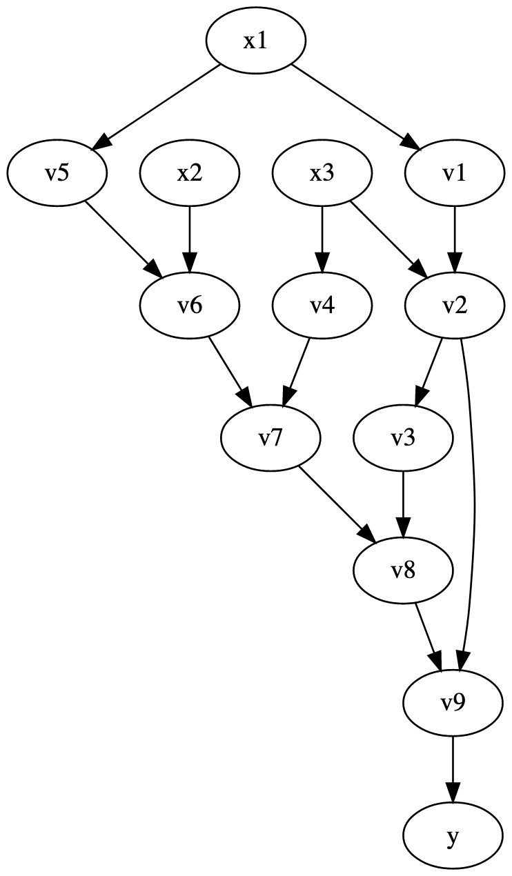
To formalize a little our graph-oriented algorithm from the previous paragraph, let's introduce some definitions. Let $f_v: \mathbb{R}^r \to \mathbb{R}$ be the function that vertex $v$ computes, and let $\partial_1 f_v, \cdots, \partial_r f_v$ be its partial derivatives that are statically known. Let $I_v$ be the vector of the vertices with an outgoing edge to $v$. Let $O_v$ be the set of vertices that $v$ has an outgoing edge. And finally let $i(v_1, v_2)$ be the index that $v_1$ is connected to $v_2$ on. For example, $f_{v_2}(x_1, x_2) = \frac{x_1}{x_2}$, $\partial_1 f_{v_2} = \frac{1}{x_2}$, $\partial_2 f_{v_2} = -\frac{x_1}{x_2^2}$. And $I_{v_2} = [v_1, v_3]$, here the order matters, since $f_{v_2}(I_{v_2})$ should be the value of $v_2$. And $O_{v_2} = \{v_3, v_9\}$, and $i(v_1, v_2) = 1$, and $i(v_3, v_2) = 2$. Then: $$ \overline{x} = \sum_{v \in O_x} \overline{v} \cdot \partial_{i(x,v)}f_v\left(I_v\right) $$

And finally, for completeness, here are the adjoints for our running example: $$ \begin{align*} \overline{f} &= 1 \\ \overline{v_9} &= \overline{y} \\ \overline{v_8} &= \overline{v_9} v_2 \\ \overline{v_7} &= \overline{v_8} \\ \overline{v_6} &= \overline{v_7} v_4 \\ \overline{v_5} &= \overline{v_6} x_2 \\ \overline{v_4} &= \overline{v_7} v_4 \\ \overline{v_3} &= \overline{v_8} \\ \overline{v_2} &= \overline{v_3} cos(v_2) + \overline{v_9} v_8 \\ \overline{v_1} &= \overline{v_2} \frac{1}{x_3} \\ \overline{x_3} &= \overline{v_4} e^{x_3} - \overline{v_2} \frac{v_1}{x_3^2} \\ \overline{x_2} &= \overline{v_6} v_5 \\ \overline{x_1} &= \overline{v_1} \frac{1}{x_1} + \overline{v_5} cos(x_1) \\ \end{align*} $$

This is all! One last observation is that in a single backward pass of $f$ we have managed to compute all its partial derivatives. Which explains why in a neural network setting reverse-mode AD is exclusively used.

To deal with $f: \mathbb{R}^n \to \mathbb{R}^m$ (since in our example $m=1$), we will have to compute $m$ different programs for each output. We can of course reuse the same trick of introducing a direction $s$ and setting $\overline{y_i} = \frac{\partial s}{\partial y_i}$. To compute all $\frac{\partial y_1}{\partial x_i}$ we just set $\overline{y_1} = 1$ and every other $\overline{y_i} = 0$.

So, when should we use each method? If we are differentiating $f: \mathbb{R}^n \to \mathbb{R}^m$, and $n \leq m$ then the numerical method is the simplest to implement, while the forward-mode AD is the fastest. And if $n > m$ then reverse-mode AD is the fastest.